🔗 Linking 2D and 3D#
Linking 2D and 3D modalities is key in various tasks enabled by our dataset, including the Grounded Compositional Recognition we propose.
We show here how to link the 2D and 3D modalities using the camera parameters and depth maps we provide in the dataloaders.
We provide the camera parameters as an \(8 \times 4\) tensor, where the upper \(4 \times 4\) matrix is the intrisic matrix \(K\), and the lower matrix is the extrinsic matrix \(M\).
from demo_utils_3D import *
from demo_utils_2D import *
import utils3D.plot as plt_utils_3D
ROOT_DIR_3D = "./3D_PC_data/"
ROOT_DIR_2D = "./2D_data/"
Projecting 3D pointclouds to the 2D image plane#
We illustrate here how to make use of the camera parameters to project 3D pointclouds to the 2D image plane.
"""
Dataloader for the full data available in the WDS shards.
Adapt and filter to the fields needed for your usage.
Args:
----
...: See FullLoader
loader_3D: The 3D loader to fetch the 3D data from.
"""
from compat2D_3D import FullLoader2D_3D
valid_loader_2D_3D = (
FullLoader2D_3D(root_url_2D=ROOT_DIR_2D,
root_dir_3D=ROOT_DIR_3D,
num_points=2048,
split="valid",
semantic_level="fine",
n_compositions=1)
.make_loader(batch_size=1, num_workers=0)
)
# Unpacking the huge sample
for data_tuple in valid_loader_2D_3D:
shape_id, image, target, \
part_mask, mat_mask, depth, \
style_id, view_id, view_type, \
cam_parameters,\
points, points_part_labels, points_mat_labels = data_tuple
break
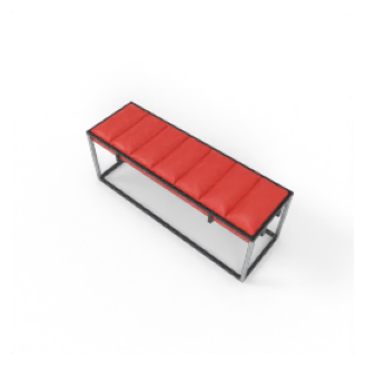
We first display the pointcloud and the rendered image, separately.
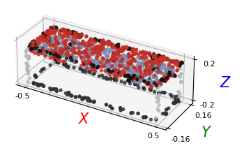
# Plotting the 3D pointcloud
points_xyz = points[:, :3]
points_col = points[:, 3:]
plt_utils.plot_pointclouds([np.array(points_xyz)],
colors=[np.array(points_col)],
size=5,
point_size=8)
show_tensors([image], size=4)
\(K\) and \(M\) are stacked vertically in the camera parameters tensor we provide. You can recover them by doing:
K, M = cam_parameters.chunk(2, axis=0)
We then project the 3D pointcloud xyz coordinates into the 2D plane, using \(K\) and \(M\). This is done simply via:
\( p_{xy} = KMp_{xyz} \)
Where both \(p_{xyz}\), \(p_{xy}\) are homogeneous point coordinates.
def project_to_2D(pointcloud, proj_matrix):
"""
Project 3D pointcloud to 2D image plane.
"""
pc = np.concatenate([pointcloud, np.ones([pointcloud.shape[0], 1])], axis=1).T
# Applying the projection matrix
pc = np.matmul(proj_matrix, pc)
pc_final = pc/pc[2]
return pc_final.T
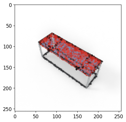
def viz_projected_points(p, image, K, M):
"""
Project 3D points to 2D image plane and visualize.
"""
# Create a new figure and axis
_, ax = plt.subplots()
# Display the rendered image
im = np.array(torch.squeeze(image).permute(1, 2, 0))
im = im/np.amax(im)
ax.imshow(im)
# Computing projection matrix from camera parameters
proj_matrix = K @ M
# Project the points to 2D
p_xyz = p[:, :3]
p_col = p[:, 3:]/255.
p_xyz[:, 2] -= np.min(p_xyz[:, 2]) # Translate points to be above the rendering plane
p_xyz = project_to_2D(p_xyz, proj_matrix=proj_matrix)
# Sample 4000 points for display
ax.scatter(p_xyz[:,0],
p_xyz[:,1],
c=p_col,
s=10,
alpha=0.25)
# Show the figure
plt.show()
K, M = cam_parameters[0].chunk(2, axis=0)
# Visualize the projected points
viz_projected_points(np.array(points), image, K, M)
Transform 2D pixels to 3D space#
Using depth maps and camera parameters, we can also transform our 2D RGB renders into the 3D space. We highlight here how to do that using the same dataloader.
Note
Values from the far clipping plane (any orthogonal distance greater than 10) have to filtered to properly make use of depth maps.
import numpy as np
def img_to_pc(img, depth_map, K, M):
"""
Convert an image and its depth map to a point cloud.
"""
depth_map = depth_map.numpy()
img = img.permute(1,2,0).numpy()
K = K[:3,:3].numpy()
# Generate the pixel grid
h, w, c = img.shape
u, v = np.meshgrid(np.arange(w), np.arange(h))
# Compute the camera coordinates of the points
fx, fy, cx, cy = K[0,0], K[1,1], K[0,2], K[1,2]
X_cam = -np.stack([(u - cx) / fx, (v - cy) / fy, np.ones((h, w))], axis=-1) * depth_map[..., np.newaxis]
X_cam = X_cam.reshape((-1, 3))
# Apply camera extrinsics
R, t = M[:3,:3], M[:3,3:]
X_world = np.dot(R, X_cam.T) + t.reshape((-1, 1))
X_world = X_world.T
# Add color information to points
points = np.hstack((X_world, img.reshape(h*w, c)))
# Reshape the points array
points = points.reshape((h * w, 3+c))
# Filter depth values from the far clipping plane
mask = (depth_map.flatten() < 10)
points = points[mask]
return points
By default, the \(M\) matrix is world-to-camera, as shown in the previous section. We must invert it before transforming points to 3D space.
M = np.linalg.inv(M)
points = img_to_pc(image[0], depth[0], K, M)
The transformed RGBD image can then be visualized:
p_xyz = points[:, :3]
p_col = points[:, 3:]
plt_utils.plot_pointclouds([p_xyz],
colors=[p_col*255.],
size=12,
point_size=8)
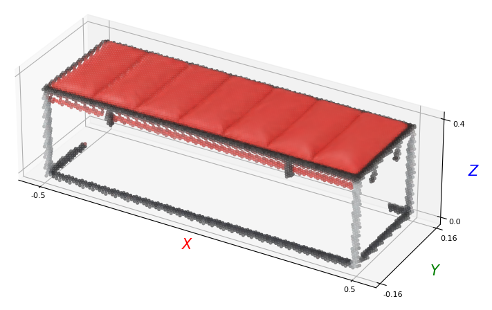
We augment the resulting pointcloud with a small additive Gaussian noise for visualization, in the interactive view below.
p_xyz_aug, p_col_aug = aug_pc(p_xyz, p_col, shift=1e-3, exp_steps=8)
p_xyz_aug = rotate_pc(p_xyz_aug)
plt_utils.show_pointcloud(p_xyz_aug, p_col_aug).show(height=300)